Fitting Critical Power model with iteratively weighted linear least squares

Now that I've establish envelope fitting can be done using an iteratively weighted least-square fitting scheme, the weights set larger for points falling above the model than below, I want to apply that approach to power-duration data.

A nice thing about this is I no longer need to partition the points into discrete regions for each model parameter. I can fit the whole curve. But I need to do that smartly.

First, there's point decimation. It's natural to plot power-duration data on a logarithmic time axis. For example, the points falling between 1000 and 2000 seconds should have about the same significance as the points between 100 and 200 seconds. Each of these sets represents a factor of two in duration difference. However, with points derived on a second-by-second basis, there would be 10 times as many points in the 1000 to 2000 range as there were in the 100 to 200 range. When doing a regression, the longer time data would thus exert far greater influence.

This can be accommodated two ways. One is with weighting: weight each point proportional to 1 / time (in addition to other weights). Another approach is to decimate the data such that they are approximately uniformly spaced on a logarithmic axis. This is arguably the better approach, since it reduces the size of the problem, and that speeds up the calculation. For example, the data can eb selected such that points occur at approximately 2.5% intervals for time points of at least 40 seconds. This will result in points less than 40 seconds being relatively short-changed in influence, but since short-time points are more prone to measurement error due to 1-second sampling, this probably isn't so bad.

The other issue is the nonlinear nature of the Veloclinic model equations. I'll worry about that later. First I want to test the approach on the simpler, linear critical power model.

The critical power model can be represented as a linear model relating work to time, as follows:
work = AWC + CP × time

Then from work I can calculate the power.

There's one subtlety with this approach, which is an additional weighting factor. As it is written, work increases approximately linearly with time. That means a given error, measured in joules, for a long time will be less of an error in power than will be the same error in joules for a shorter time. This essentially places a priority on matching long-time points. To correct this error, an additional weighting factor is needed of 1 / time squared. The square is because the weighting factor is applied not to the error but to the square of the error.

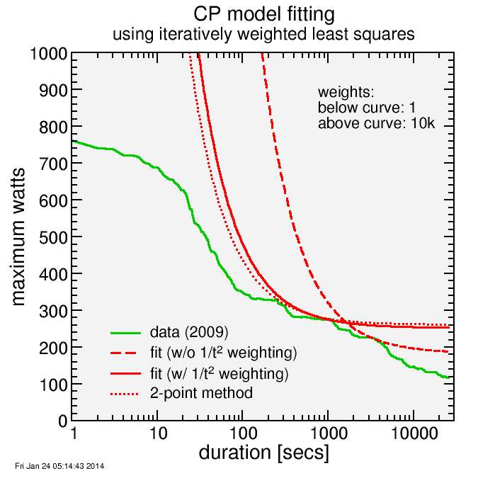
Here's a result. I show two fits, one with the inverse time squared weighting factor, one without. The one without the weighting factor produces an inferior fit where it's wanted, which is in the range of 10 minutes to maybe 30 minutes where the CP model should work well. Also added to the curve is the 2-point method I developed for Golden Cheetah. The 2-point method finds two quality points, one in the anaerobic zone, one in the aerobic zone, and runs the CP curve through those.

With the 1/t² weighting, the regression method gives a similar curve to the 2-point method, with a slight shift from CP to AWC.

Next would be to apply this method to the Veloclinic model, which is nonlinear.