automated fitting of the VeloClinic model: fail
I developed an automated fitting algorithm for the Veloclinic power-duration model, or rather the variant that I described in this blog, with the addition of a square root term on the time dependence of the aerobic power. Or at least I tried.
First I test it against the model itself. I first created an "ideal" power-duration curve with the following Perl snippet:
  my @pmax;
  for my $t ( 1 .. $duration ) {
    push @pmax,
      $P1 * ($tau1 / $t) * (1 - exp(-$t / $tau1)) +
        $P2 * sqrt($tau2 / $t) * (1 - exp(- sqrt($t / $tau2)));
  }
Then I created 3 hours of ride data and ran it through my fitting program. The plot is from my "quick and dirty" plotting program of choice, xgraph. The axes aren't so clear: the "x-axis" is time in seconds on a logarithmic scale, and the "y-axis" is power in watts.
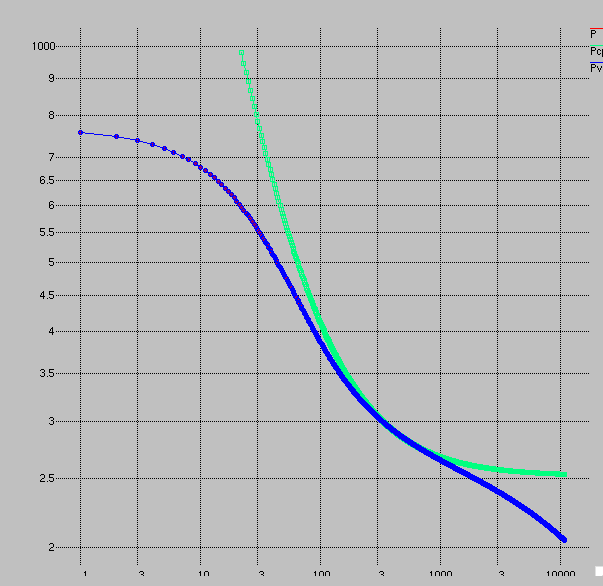
Two fits are shown, one for the CP model and the other for the Veloclinic model. The fit to the Veloclinic model is essentially perfect: the curves overlap. This is of course because the data were generated with the same model. But at least the fitting program is working in the easiest case.
The CP model, of course, does a poor job except over a very small range of ride durations. This is because it assumes aerobic power can be sustained forever, and it assumes anaerobic work can be fully utilized instantly. Neither of these assumptions is close to correct.
Here's a comparison of the fitting parameters:
| parameter | actual | fit |
|---|---|---|
| P1 | 490 | 490.005 |
| τ1 | 24 | 24.007 |
| P2 | 280 | 279.98 |
| τ2 | 24000 | 24029 |
So the original model parameters are reproduced with excellent precision: no worse than 0.12%. Three of the four parameters are much better than this. But this doesn't prove anything about the quality of the envelope fit. All of the points fall on the curve, effectively, so even an least-squares fitting scheme would have done as well.
Next step I fit to partial data again taken from the same model. In this case instead of every point on the curve being power from the model, I assume the rider did a finite number of rides of different duration, each ride "optimal" for that duration given the model. This is a test of the envelope fit. The goal is that the ride durations fall on the curve, but all other durations fall below the curve due to a lack of optimal efforts.
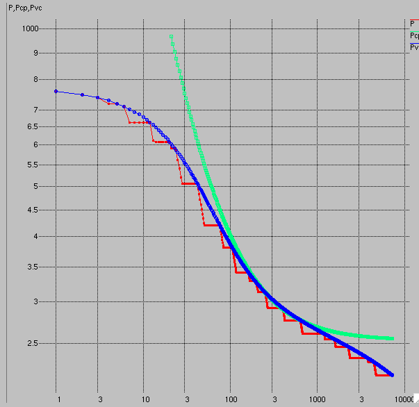
Here's a comparison of the fitting parameters:
| parameter | actual | fit |
|---|---|---|
| P1 | 490 | 490.003 |
| τ1 | 24 | 24.004 |
| P2 | 280 | 279.991 |
| τ2 | 24000 | 24011 |
Surprisingly, these are even better than last time. But maybe it isn't surprising: it was forced to pick points with which to fit the model which are relatively spread out. But hindsight is 20:20.
It's looking really good now, right? But wait... I dredged up some old data from my 2009 pre-Strava days. Crash and burn:
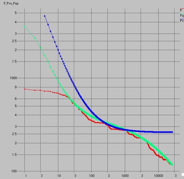
The fit is fine for much of the curve, but drastically overestimates maximum power. Indeed, the time constant for anaerobic power from the fit is only 1.24 seconds, with a maximum power for this component of 4.6 kW. The product is 5.7 kJ, a reasonable number for AWC, but the peak power is too large, and clearly the "fit" to small powers is poor. Yet if I were to force the algorithm to fit this section better, the results wouldn't be much more satisfactory.
What I do for this fit is to sequentially examine sections of the curve, and use each to optimize a particular parameter which is relatively more important for that portion. I start by fitting the CP curve. This gives me two parameters: CP and AWC. I then set P2 = CP. For P1, I use the one-second power, subtracting off CP. Then I set τ1 = AWC / P1. I assume τ2 = 24000, which seems a reasonable guess based on having done a hand fit to a plot of superposed power-duration curves from my own records.
So I then go through each parameter in turn. I start with P1. I look for points in the range from 5 to 30 seconds, picking the one which gives me the maximum value of P1 needed to match that power point, all other parameters fixed at the previous guess. Then I go to the endurance side. I look at points from 3600 to 5400 seconds, stepping by 5 seconds, looking for the point which gives me the maximum estimate of τ2, all other parameters fixed. Then I move back to the anaerobic portion of the curve, from 60 to 360 seconds, looking for the point which gives the highest value of &tau1. Finally I look at the "aerobic" portion, from 600 to 1800 seconds, looking for the point which gives me the highest value of P2. I repeat this sequence until the numbers stop changing to a summed relative difference of 0.01%. For this curve, this took 27 iterations.
The "quality points" which result from this process in this example are at 22, 60, 1076, and 3600 seconds. Four quality points allow setting of the four parameters.
But as you can see it didn't work so well. If you were to see this data fit in Golden Cheetah you'd want your money back. Confidence in the fit is necessary to draw lessons from the results.
One point of interest in the fit is the range from 200 to 1000 seconds. Here the Veloclinic model predicts a higher maximum power than the CP model. More typically, by virtue of providing additional constraints, the Veloclinic model predicts lower power, but in this section, the predicted power is greater. Suppose you feel fresh and ready to go and want to absolutely drill a 10-minute (600 second) effort. Do you pace it off the CP model or the Veloclinic model? If I choose CP, I go out at 290 watts. On the other hand, if I choose the Veloclinic model, I go out at 300 watts. That's potentially a big difference.
The reason for the higher Veloclinic model prediction is the model is assuming a relatively high rate of fatigue on aerobic power: the fitted value of τ2 is only 2961 seconds. That's obviously a lot shorter than I'd fit for an aggregate superposition of power-duration curves from my pre-Strava files. It happened to be the case in this data set I'd done no quality efforts over an hour, and I use efforts over an hour to determine τ2. So it assumed my lack of good numbers wasn't due to lack of effort, but rather due to lack of ability, and therefore my promising aerobic power in the 18-minute range (1076 seconds) simply wasn't up to the task of producing power for 3600 seconds. But this high rate of decay for times over 18 minutes implies a high rate of ride for times less than 18 minutes. So this boosts the prediction for 5 minutes. In reality, I trust CP more.
So good, robust fitting is important, and I don't yet have confidence in the fitting scheme I have, no matter how well it did on toy data.
So what to do? One approach I tried is to add an additional component, P0, which caps the power at very low durations. Then I modified the the power from the existing model with the following heuristic equation:
Pnew = [ P0−5 + PVC−5 ]−1/5
But I'm not going to promote this without justification, especially since it's not integrated with my fitting function, but is applied post-process.
So the question is why the fit is so poor. I think the answer is my fitting scheme is too simple-minded. I fit each parameter in turn, using different segments of the data, the goal of each being to maximize its value. I think I need some sort of global goodness-of-fit metric. For example, since I want an envelope fit, I am much more sensitive to points falling above the model curve than below, but I still care about points falling below. Additionally since it's natural to plot the data with logarithmic axes, I want to weight the points by 1 / (t × P), or weight by 1/P and decimate the points to constant spacing of the logarithm of time (which will save computation time). Least square fits are done with an error function of error-squared, but since I want the envelope, a strongly asymmetric error function would be needed. Anyway, these are just ideas.


Comments