2013 Low-Key Hillclimbs: examining the score algorithm

With the 2013 Low-Key Hillclimbs now over, it is a good chance to reflect on the scoring scheme and to see if it accomplished its goal of making similar relative performances on substantially different climbs score similarly.

To check this, I took the score from each week and adjusted it for the quality of the riders on that week. This should in theory result in a similar scoreing distribution as if riders of similar speed showed up each week. The rider quality adjustment is done to scores if primarily faster or slower riders show up certain weeks. For example, particularly challenging climbs like Montara tend to attract primarily stronger riders.

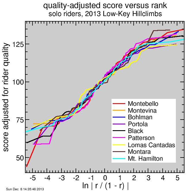
Then I plotted these scores versus rank. I used a normalized rank r which goes from 0 to 1, then applied a log-normal transformation to that number to map 0 to 1 to -infinity to +infinity.

Each week is scored using two adjustable parameters: a reference time and a slope factor. The goal of these parameters is to make each rider's scores during the series as tight as possible. The slope factor is needed because on some climbs, like Mount Hamilton, riders tend to finish relatively closer together due to the influence of the descents and on packs riding together up the first of the three climbs. Other climbs, most notably Portola Valley short-hills, riders tend to finish with a relatively larger spread of times. The 7x challenge, including the super-steep Marin Ave, also had a relatively broad spread of times, due no doubt to the fact some riders were forced to climb in survival mode up Marin.

You might think the slope factor would result in each climb having a similar score-versus-rank curve. This is similar, but not identical. Nor should they be identical: if they overlapped that would mean rank and only rank counted. If riders finish in a group I want them to have similar scores. Groups create plateus on a plot of score versus rank. But generally I want the curves to be such it's hard to differentiate one climb from another, except for plateaus.

Here's the result.

Montara was remarkable for some very high scores. But you can see from the plot that it's only the top 2 scores which are unusual. Montara attracted two particularly good dirt riders, and they finished close together, so it's appropriate they scored highly.

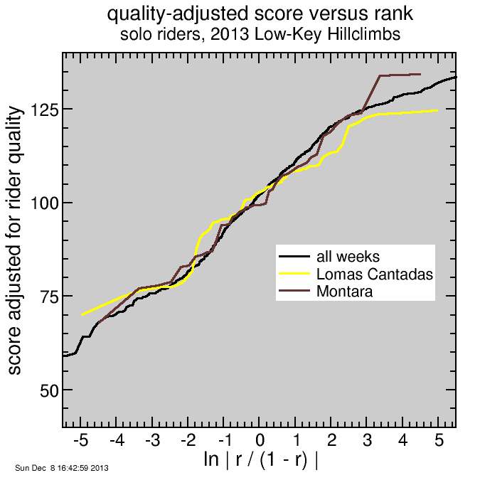
Actually the only curve which looks a bit weird there is Lomas Cantadas. I'll need to look into that. Here's the curves for Lomas Cantadas, Montara, and the aggregate curve from combining all weeks. It seems Lomas is a bit flatter than the others.

I thought perhaps this is due to the influence of so many one-time riders, 12/72, who failed to contribute to the slope term since the code had no basis for comparison for them since they did only one climb. So I recalculated the Lomas curve with only returning riders and plotted it as a dashed line. That is a bit better, but not much:

So I take a step back and look at the code, which I wrote back in 2011 for the "score slope" factors. Does it make sense?

sub iterate_score_slopes {
  for my $w ( @weeks ) {
    my $sum0 = 0;
    my $sum1 = 0;
    warn("iterating reference time for week $w.\n");
    # sum of the squares of the deviations of log scores from ratings
    for my $r ( @{$week_riders{$w}} ) {
      if ( $rider_statistical_weight{$r} > 0 ) {
        $sum0 += $rider_statistical_weight{$r} * $rider_rating{$r} ** 2;
        $sum1 += $rider_statistical_weight{$r} *
          log($reference_time_eff{$w} / $rider_time_eff{$w}->{$r}) ** 2;
      }
    }
    $score_slope{$w} = sqrt($sum0 / $sum1)
      if ($sum1);
  }

  # normalize score slopes
  $sum0 = 0;
  $sum1 = 0;
  for my $w ( @weeks ) {
    if ($score_slope{$w} > 0) {
      $sum0 += $week_statistical_weight{$w};
      $sum1 += $week_statistical_weight{$w} * log($score_slope{$w});
    }
  }
  if ($sum0) {
    for my $w ( @weeks ) {
      $score_slope{$w} = exp(log($score_slope{$w}) - $sum1 / $sum0)
        if ($score_slope{$w});
      warn("normalized slope for week $w = $score_slope{$w}\n");
    }
  }
}

The key here is it is calculating a rating for each rider based on all of his results, then checking that the deviation of the rider's scores from that rating is minimized. This explains the shallower slope of the curve for Lomas Cantadas. It's not that the algorithm failed to yield the same curve, but that the riders who showed up for the climb were more similar (as judged by how they did in other climbs) than riders for other climbs tended to be. So the algorithm is good. To have tried to spread out the scores for Lomas more than they were, comparable to the spreads of scores from other weeks, would have been artificial, since the riders were of more similar abilities than climbs of other weeks.

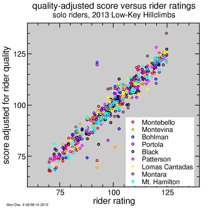
So here's a plot of rider scores plotted versus the rider rating. This plot only makes sense for riders who've ridden at least two climbs, otherwise their rating equals their single score. The goal of the scoring is to have this cloud be as tight as possible with the two adjustable parameters per week.

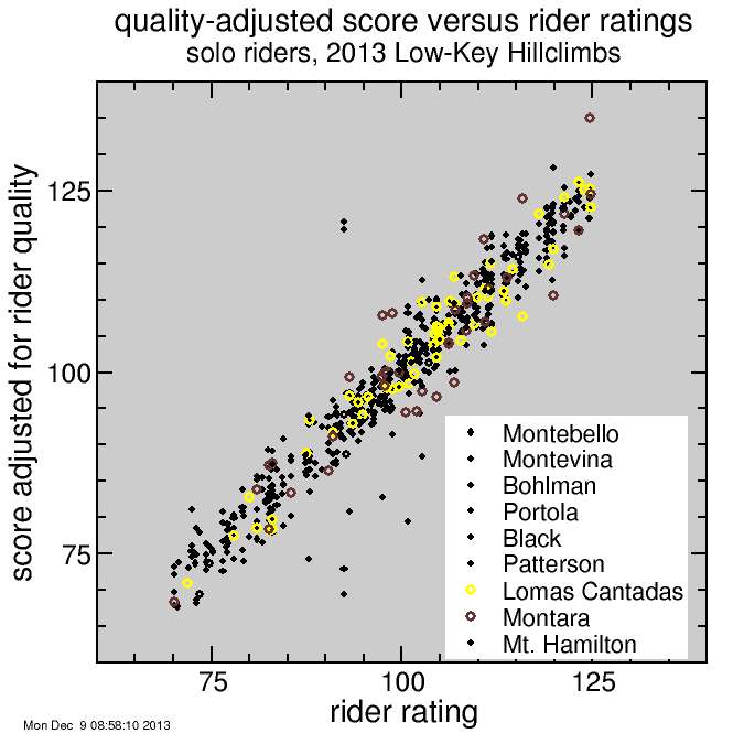
It's a cluttered plot, so I isolate the two weeks of primary interest here:

Montara resulted in scores which deviated from rating more than most weeks, as expected, but here Lomas Cantadas seems quite typical. You can see David Collet's big score from Montara (brown point) but not Keith Hillier. Keith isn't shown because this was the only Low-Key he did.

In any case, the conclusion is in particular for Montara the scores were not anomalously high. There were two exceptional dirt riders there and they scored exceptionally highly. Was dirt too much of an influence on the series this year? I think it was a relatively high influence relative to past years, but part of the fun of Low-Key, like other races such as the Tour de France, is it's a bit different year to year. Just like the 2011 Tour was affected by the cobbles of Paris-Roubaix, an atypical influence, and the Tour of 2014 will feature an exceptionally long time trial, we can't expect every year to favor the same riders in Low-Key Hillclimbs.