Converting Run Times to Cycling Times for Low-Key Hillclimbs: Part 3

Last time I described the procedure for constructing a look-up table for time conversion for road segments of a particular road grade. The road grade is the result of taking the route profile for a course, extracted for example from barometric altimetry + GPS data (Garmin Edge 500, Garmin Edge 800), and convolving it with a smoothing function to reduce grade changes which occur over substantially less distance than 25 meters. The approach is based on an equation fit to data from Minetti, et al, published in the Journal of Applied Physiology in 2002.

Here's the model, where metabolic cost is measured in energy per unit distance. Although metabolic heat is more conventionally reported in calories, I prefer joules in order to facilitate conversion between power, work, and heat. I assumed running for grades up to 12%, and walking for grades larger than 12%, which is consistent with my typical practice (perhaps not Gary "the" Gellin, who could run up a sheer vertical wall and still do sub-9 minute miles).

dE/ds =
a₀ +
a₁ (g' + g'₀)² +
a₂ (g' + g'₀)⁴ +
a₃ (g' + g'₀)⁶

where I define:

g' = grade / sqrt[ 1 + grade² ]

and where I derived the following heuristic model parameters:

a₀ = 1.68 J/m/kg a₁ = 54.9 J/m/kg a₂ = −102 J/m/kg a₃ = 200 J/m/kg g'₀ = 18.4%

To convert cycling power to metabolic cost, I assumed a 3% drivetrain loss rate, and I assumed a cyclist metabolic efficiency of 25.7%, which is the lowest value which avoids the bike rider requiring a greater rate of metabolic cost than the runner at the same road grade given the idealized assumption of zero bike weight and zero drivetrain efficiency. However, here I take a slightly different approach.

The retarding force from wind resistance is typically modeled as 1/2 ρ Cd A v², where ρ is the air density (typically approximately 1.15 kg/m³), Cd is the coefficient of wind resistance, A is the cross-sectional area, and v² is the square of the bike or runner speed. For the cyclist, I am going to arbitrarily assume a CdA of approximately 0.45 m² per 75 kg of body mass, while for the runner, I will assume Cd of approximately 0.8 with an area of approximately 0.75 meters squared, totalling 0.6 m² for the same 75 kg of body mass. So the runner, by virtue of an upright position, will have more wind resistance, and will typically be wearing less aerodynamically efficiency clothing, although he is spared the wind drag of a bicycle. For runners, the key question is how to convert this wind drag to merginal metabolic cost. For that I can just assume a marginal metabolic efficiency. 25% seems a good choice, so that's what I used.

For cycling, I assumed a CdA of 0.45 m² for a 75 kg cyclist. I estimated a rolling resistance coefficient of around 0.4%. I set extra mass, including bike and clothing, to a modest 12% of the body mass (9 kg). I then assumed the cyclist could sustain 5 W/kg, which yields an Old La Honda time of just over 17 minutes.

As I noted last time, I asserted at high speeds the cyclist is retarded by safety considerations, which I applied as follows:

v → (v⁻⁴ + vmax⁻⁴)^−1/4 .

Here's the resulting pace in minutes / km (I like min/km ore than min/mile because it makes calculation of times for 10 km races simple, perhaps except for a fractional minutes-to-second conversion):

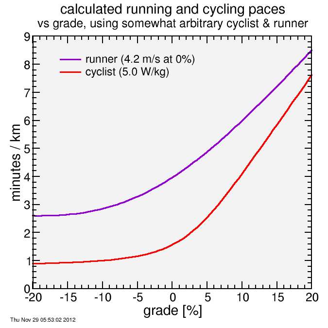
calculated minutes per km for model cyclist and runner. I assume the runner can do just under 4 min per km (4.3 meters/second) while the cyclist can sustain 5 W/kg (17-minute Old La Honda). I then scale runner speeds using my analytic fit to Minetti's metabolic cost data, adjusted for estimated wind resistance with a 25% metabolic efficiency. For the rider, I assume a climb-like bike position for wind resistance with 12% of total weight taken up by the bike + clothing.

As expected, the cyclist at negative and zero grades has a substantial advantage, but as the road gets steeper, the runner does better relative to the cyclist. Here there is no cross-over point, unlike my last calculation where the conversion between runner and cyclist was based on an assumption of metabolic efficiency However that approach substantially overestimated what speed I would be able to sustain up Old La Honda, so for this calculation the more heuristically based criteria for setting cyclist and runner speeds independently (I still used a metabolic efficiency for the small correction to runner speed due to wind resistance in still air) resulted in lower running speeds, and therefore the cyclist in this case is able to sustain an advantage to the 20% in the plot.

It appears from the trend as if the runner will eventually catch up to the cyclist pace but in fact this isn't the case due to the nonlinearity in the metabolic running cost with road grade. This is optimistic about the ability to sustain power on a bicycle at extreme grades, however. Eventually traction becomes an issue, and likely gearing becomes limited, unless you're riding a bike like Dan Guttierez's Fargo-Road-climbing-custom (video). But then who says you're not? My model shouldn't assume you're riding an inappropriate machine for the road.

Anyway, I then calculated a score conversion factor for running scores. As I noted, rather than rely heavily on my ad hoc assumptions about what speeds a model runner versus a model cyclist can sustain, I constrained the score conversion to 1 at a 12% grade. The result is here:

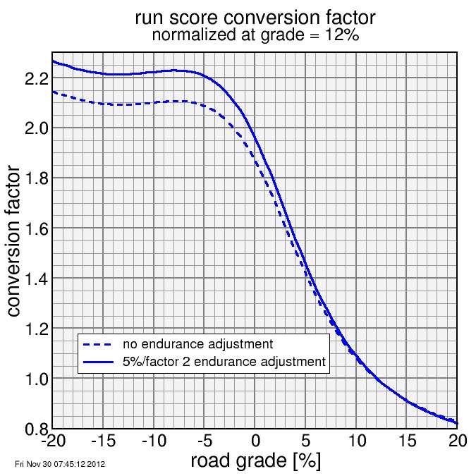
Score conversion factor for runners versus road grade. Actual roads will be adjusted on a segment-by-segment basis using full profile data (with Gaussian smoothing). While specific assumed cycling and running speeds were used to generate this curve, the effect of these assumptions was only on wind resistance, and therefore for climbs the affect on the conversion factor is small. The dashed line is for equal time, the solid line adjusts for the runner taking more time and thus facing greater fatigue than the cyclist (for the grades on the plot). Each curve is independently normalized to 1 at a 12% grade.

What I'm missing in the dashed line in this plot is the effect of endurance, however. I started by assuming cyclists could sustain a given power and runners a given flat road pace, but of course they can't do that indefinitely. However, such a pace cannot be sustained indefinitely. Looking at world record times, there is a trend that these speeds fall around 5% every time the time required is doubled. I can model that as speed is inversely proportional to distance (at a given grade) raised to the power ln(1.05)/ln(2). There's a minor issue whether the 5% applies to doubling of distance or time. I'll assume time. That means to get an exponent to apply to distance I need to solve self-consistently, which can be done analytically via the transformation of the exponent k

kd = kt / (1 - kt )

where kt is the exponent for time and d is the exponent for distance. So in my application speed is changing over the course due to grade, but on constant grade I initially assume constant speed, so instead of kd here I can use initially calculated time. So what I do for endurance is to take a reference time at which the assumed flat-pace or power can be sustained, then assume that pace applies to any distance, then once I've calculated a power I multiply it by the ratio of the initially calculated time to the reference time raised to the power calculated to yield my 5%/factor-of-two-time speed loss, which is 0.0757.

The effect of the endurance adjustment is shown as the solid line in the preceding plot. For relatively flat or descending routes, the runner takes more time relative to the cyclist than he would on the reference 12% grade, and therefore his speed will be relatively degraded by the assumed 5%/factor-of-2-in-duration rate of decay. The effect is 5% total for when the conversion factor reaches 2 (which is what it is designed to do).

So that's it. All I need to do next is test it on a real hills.