simulating effect of grade variations on climbing VAM

One issue in using VAM to predict power is the effect of variation in grade. I looked at this back in November, 2009. Grade variation leads to speed variation (at constant power) and speed variation results in an increase in energy dissipated to wind resistance. The analytic result I got was:

Δp / p₀ ≈
3 f [ <Δgrade²> / (grade₀ + C_RR)² ] × [ ( 1 - f ) / ( 1 + 2 f ) ]²

where f is the fraction of power from wind resistance, <Δgrade²> is the variance of grade with respect to time (this is to first order the variance with respect to position), and C_RR is the coefficient of rolling resistance. Using iBike data from a ride up Old La Honda (iBike directly measures grade, rather than indirectly via altitude), I concluded at constant power up Old La Honda the grade variation would lead to a 0.44% increase in power.

I can convert this to the effect on VAM by multiplying by the fractional effect of power on VAM:

ΔVAM / VAM₀ ≈
3 f [ <Δgrade²> / (grade₀ + C_RR)² ] × ( 1 - f )² / ( 1 + 2 f )³

This is a bit indirect so it's important to review the assumptions:

1. A rider is riding at constant power up a climb. This yields a certain speed variation associated with a certain grade variation.
2. The speed variation is going to yield a certain power increase due to wind resistance relative to riding at a steady, average speed.
3. The rider is riding a constant power, so higher required power must be canceled with a reduction in average speed.
4. Lower average speed reduces average VAM.

The reason this came up is the recent widespread interest in the use of power analysis to assess the likelihood of rider doping in the Tour de France. If you estimate power using certain assumptions, it's important to assess the error introduced by those assumptions.

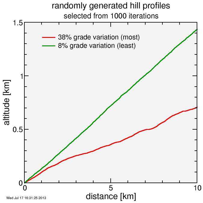
So I decided to test this, which took only a few minutes with the script I wrote for the preceding analysis of pVAM. I wrote some simple code which picked a random grade and a random fractional grade variation for a 10 km climb which I divided into 100 equal-grade segments of constant grade. For each new segment, I picked a new random grade, but because grade is locally correlated, I did a weighted average of 3-parts previous segment grade to 1-part this newly selected grade. This created hill profiles which looked realistic to me. The average climb had a 7.5% grade with an 18.3% grade variation, although both the grade and the variation in grade varied substantially. I simulated 1000 climbs this way.

Here's some sample profiles. Of the 1000 iterations, I plot the profiles with the least and greatest fractional variation in grade. They pass the "looks real" test to me:

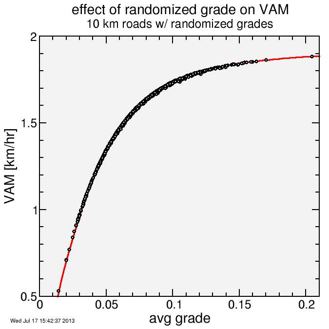
Here's the VAM versus average grade (points) plotted against the result for a constant grade (red line). I didn't use the critical power model here, but rather assumed a constant power of 6 W/kg (Powertap power).

The VAM numbers are close to those for a constant grade of the same average. To see that a bit better, I plot the % VAM reduction due to the grade nonuniformity here, using a fresh set of 1000 hills (these points don't correspond to those in the previous plot):

The result is consistent with that analysis from 2009: the grade variations reduce the VAM by a fraction of a percent. The plot brings out an interesting aspect of the equation: very low grade, and wind resistance dominates, and grade doesn't affect speed as much, while very large grade, and wind resistance is less relevant, so speed fluctuations don't matter much. The effect, though small, isn't unbiased: the VAM is always reduced, never increased, by grade variations. But the error from neglecting grade fluctuations is small compared to other error sources, in particular the wind (as was recently pointed out by Alex Simmons).

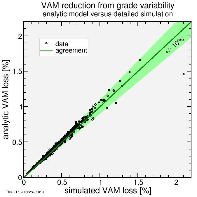
I also checked the result of the detailed simulation against the analytic equation. As you can see in the plot, the analytic equation is generally good to within 10% of the detailed simulation result. The notable outlier contained a short descent and obviously exceeded the low-order analysis used. Note the plot is showing the fractional reduction in VAM due to the grade variation, not the fractional error in VAM. That would be much less, since the total reduction is typically on order 0.5%.