Calibrating Heuristic Bike Speed Model to 2011 Terrible Two winner

For the Terrible Two, I used data from Adam Bickett, who finished first (PDF results). A fast rider is good for model validation because he paced himself well and minimized rest time. The model doesn't include consideration of rest or recovery.

Rather than do any formal fitting, I fit "by eye". To do this I examined VAM (rare of vertical ascent), speed, and time relative to schedule, all versus distance.

The resulting parameters were the following. I won't attempt to assign error bars:

vmax	:	17 m/s
v0	:	9.5 m/s
VAMmax	:	0.52 m/s
rfatigue	:	2%/hr

I didn't try to fit the cornering penalty, which I kept at 40 meters / radian, and which seemed to work fairly well. Note the VAM number is comparable to Contador on Spanish beef, but this is climbing in the infinite-sine-angle limit (mathematically impossible) and actual VAMs produced by the model are substantially less.

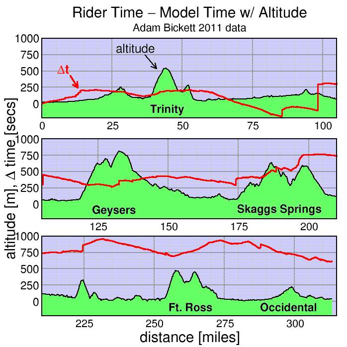
First I plot how the time to a given point on the course compares between the ride data and the model (red curve, in seconds). In the plot, positive values imply the rider was slower to that point than the model predicted, while negative values imply the rider was faster. The black curve with green fill is the course profile, in meters. Click on the plot to expand it.

The start is neutral and the rider started out a bit slow, losing around 3 minutes in the first 14 km. Then the model did a good job matching the data through the climb and descent of Trinity Grade. On the flats pacelines can really fly, and the rider gained close to 4 minutes versus the model through 85 km. The rider stopped for 2 minutes then rode to km 98 where he stopped for 6.5 minutes, rode at close to model pace for 5 km, then stopped again, this time for 2 minutes. He then stays within 2 minutes of modeled pace to the lunch stop at 174 km.

His stop here was extraordinary, just 1.5 minutes, then he tackled Skaggs Springs Road. The model somewhat overpredicts his climbing rate here, since he lost time on the climbs, around 6 minutes to the next rest stop where he stopped for only 1 minute. He then lost another 1.5 minutes off the modeled pace out to the coast. But ride down the coast is usually a tail wind and it appears 2011 was no different: he flew down the coast well faster than schedule, gaining back 4.5 minutes. Fort Ross went well: he lost only a minute, but the descent from Fort Ross is on rough roads and he descended these slower than the model predicts (it knows nothing of road conditions). He recovered a bit by the final rest stop where he was remarkably brief (around 50 seconds) before jamming it ahead of model pace the rest of the way to the finish.

Overall he finished 10 minutes slower than the calibrated model. He spent close to 20 minutes total stopped, so his overall ride pace was 10 minutes faster than the model, all of that attributable to his speed down the coast and from the final rest stop to the finish.

Of course this isn't validation of the predictive aspect of the model since I crudely fit the coefficients to match these data. But the model, with resonable coefficients set to rough precision, does seem to capture the rider's behavior over the course of the ride and on the different terrain fairly well.

Next to gain further insight I turned to rate of vertical ascent (VAM). For most analysis I used meters/second for speed, but for VAM I more often defer to the more traditional meters/hour. The model without fatigue and, to a lesser extent, turning penalty would assume a fixed VAM as a function of grade, but with fatigue climbs along different portions of the course yield different VAMS (later = slower). After data smoothing I decimate the data to 10-second time spacing, to avoid clutter.

Here's the VAM versus grade.

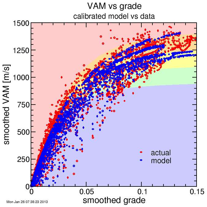
In the background of the plot I put color contours corresponding to various estimated ride powers: less than 3.0 W/kg (blue) to more than 4.5 W/kg (red). It's hard to see, but these contours track the actual data worse than the heuristic model.

To investigate this further, I plot power versus road grade. The rider had a power meter, so power is measured directly. I smooth power in the same way I smooth altitude (and implicitly road grade) to maintain a proper correspondance. I also calculated power from the heuristic speed model. This required certain assumptions. I assumed C_RR = 0.3% (roughly fit to data), C_DA = 0.45 m², rider mass = 77 kg (fit to data), bike mass = 8 kg (a bit heavy, but I assume a pump and tools and partially filled water bottles), and extra mass = 2 kg (clothing, shoes, helmet). All that matters is total mass, so maybe rider mass is a few kg high but bike mass is a few kg low. I neglected inertial power since the heuristic model can predict artificially high accelerations coming out of corners (it's designed more for speed than accurate accelerations). I model air density exponentially decaying with altitude but that's insignificant on this route. I assumed still air for now.

First, it's clear the explanation for the relative failure of the constant power assumption is the rider isn't riding constant power. His data generally increase with grade. For negative grades, he typically coasts (near-zero power) while for grades over 10% his power is solidly high. The heuristic model combined with the analytic bike power-speed model captures this behavior very well. It's important to remember that the heuristic model has nothing to do with the bike power-speed model. It simply tries to match typical behavior in speed. It's more common to model speed based on assumed power, but here I model speed directly, and from that derive power.

Note, however, that the power at near-zero grade and for descents to -5% the model yields higher powers than the rider data. Since I intentionally matched the flat-road speed to the rider's flat-road speed this isn't a matter of the heuristic model making different assumptions about rider behavior but rather the power-speed model not accurately describing the riding conditions. The most obvious source of this inaccuracy is the zero-wind assumption. It was already noted the rider went quickly south along the coast, so I simply modeled this with an assumption of a north wind at a relatively modest 3 m/sec. Here's the result:

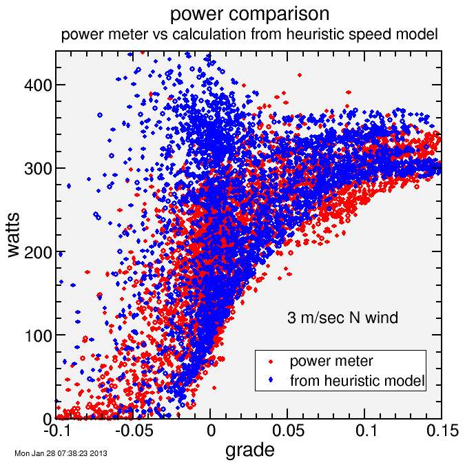
Now there's a surplus of points near zero grade with higher powers than were measured. However, the trend is much better. The obviously simplification is the assumption of constant wind over the entire course as the rider traversed it. But I'm not going to try and model time-and-position-dependent wind.

This takes care of climbing, but what about descending? My a priori assumption on descending was riders tend to ride to a certain safe speed but no further, until for grades steeper than -10% they slow. This is in contrast to the "terminal velocity" model where a coasting rider's speed will inrease proportional to the square root of the sine of the road angle (which is close to road grade). I need to check that this assumption is consistent with the ride data. Here's a plot of speed versus grade, highlighting the speed of negative grades:

You can see that indeed the rider behaved much like the heuristic model assumes. At grades much steeper than -10%, the speed drops.

All of this has validated that my relatively simple heuristic model is reasonably capturing the behavior of an exemplary cyclist on a hilly course. It seems like a fantastic stroke of luck since the formula I used has no basis in physics. But it's not luck: the reason is the model makes reasonable assumptions about hills (approaching constant VAM), descents (approaching constant speed), steep roads (decreasing speed when the road gets super-steep), then connects these extremes with an analytically smooth function. I put in an additional fitting parameter to match the speed on flat roads. Then I add a fatigue term and a small correction for curvy descents and that's basically it. The primary issue is I don't capture the effect of different conditions on different portions of the course. But the goal is simplicity and universality at the expense of precisely matching data for a particular rider on a particular course on a particular day.

If I were going to extend the model I'd probably add wind effects and road condition effects.

Wind would affect v₀ only: gusting winds can affect the safe cornering speed, for example, but steep climbs tend to be shielded from the wind, and descending at the safety limit isn't systematically affected by steady wind. It's flat roads and gradual grades which are primarily affected, and v₀ takes care of that. So it would need to be made a function of heading for the wind at a particular location on the course. For example, for Terrible Two, I might model a wind based on a proximity from the coast, which can be modeled geometrically.

Road conditions would affect all three: v_max, v₀, and VAM_max. For example, a dirt or heavily graveled road both increases the power for a given flat or climbing speed and affects the safe descending rate.

These enhancements would improve the fit to the Terrible Two data. But for most purposes, I think the present model strikes a good balance between simplicity and accuracy.