Applying speed model to Terrible Two and testing cosine-squared grade distribution

Previous post I applied a heuristic power-speed model to a simple distribution of road grades. Instead of assuming grades are normally distributed, I assumed they are distributed proportional to cosine-squared. The cosine-squared distribution goes truly to zero. Since the normal distribution is characteristic of random processes, per the central limit theorem, it's widely applicable, but roads are designed and not random, so it's reasonable to expect a deviation from normal.

With this distribution, each set of similar roads is described by a parameter, g_max, which is the maximum grade encountered. I decided to apply this to Terrible Two to see what I get.

I use 2011 Strava data from Adam Beckett, who road a blazing fast T2 with minimal rest stops. Data from fast riders is best, because they are least likely to have traversed on steep climbs, and that would reduce the apparent grade. They additional are least likely to have spent time in rest stops, and moving back and forth in rest stops provides further misleading data.

I smoothed the data with a 50 meter biexponential smoothing function (50 meters of road distance). This reduced the effect of altitude errors and yet retains any hills of meaningful duration (less than 50 meters can be facilitated with inertia). I then resampled it at 50 meter intervals. I then generated a histogram with 1% bins. Here's the result:

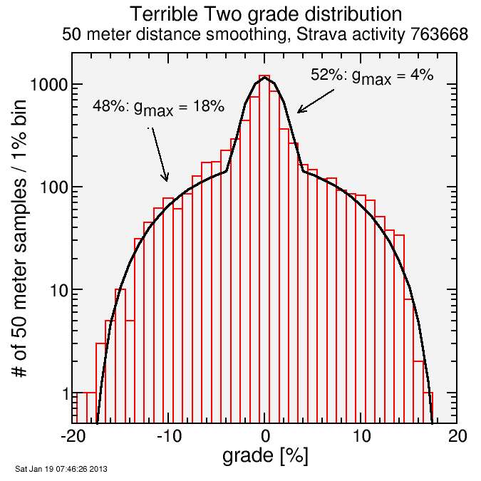
You can see the cosine-squared distribution doesn't fit the data globally, but two such distributions superposed does a very good job by qualitative assessment. 52% of the distance is characterized g_max = 4%, and 48% is characterized with g_max = 18%.

My fitting here was quick and crude and "by eye". In retrospect I think the steep portion is slightly underweighted and the flat section slightly overweighted. But this is just a rough analysis.

This bimodality is consistent with perception on the Terrible Two course: there's a lot of relatively flat and a lot of brutally steep. Combined they yield the combined statistics of, using what Strava reports: 313.1 km with 5,476 m climbing. Note this is a bit less than 200 miles, which is well documented. The course was shortened relative to the original. 313 km is quite enough, I assure you.

Applying my formula to these distributions is likely optimistic since the descents on Terrible Two are relatively slow due to the frequent corners and exceptionally rough Sonoma County asphalt (and in places no asphalt). On the other hand, the section on the coast has typically a considerable tailwind not balanced by any strong headwind sections, so this partially balances that error.

On the steep section, I get δ = 0.491 (the fractional time increased versus a flat road). For the flatter section, I get 0.036. A weighted average (48% steep, 52% flat) yields 0.25. SO Terrible Two should take around 25% longer than a flat route at the same general pace. But going 25% further tends to increase fatigue. Assuming 5% slower per 2x increase in time, this increases to 27%. So the model predicts Terrible Two should be around 27% slower than a flat course, neglecting the asphalt, turns, and winds. This seems about right.