exponential filter impulse response for altitude data smoothing
Linear filters are characterized by their impulse responses. To test my exponential filter algorithm, I created an input data set with zero-value points randomly spaced in time. At zero I put a finite approximation to a unit impulse:
‒0.01, 0
0, 100
0.01 0
I then ran this through my exponential filter in various ways.
One way is to run the points in time-forward order. This is the "causal" approach: I'm analyzing data as it comes, and I want a smoothed result as I am receiving data. Also causal is to run the smoothed curve again through the exponential filter. You'd expect this second smoothed result to be even smoother than the first time through, and of course it is.
Then there's a single and double application of the exponential filter in reverse time order. You'd expect the result to be flipped from the forward-time order (there's nothing special about forward time versus reverse time which should make the shape different; if it were there'd be something wrong).
As a third option, I do the filter in forward time and in reverse time, separately, and average the two results. This is very similar to running the filter for forward time and then running that smoothed result in reverse time.
Here's the results:
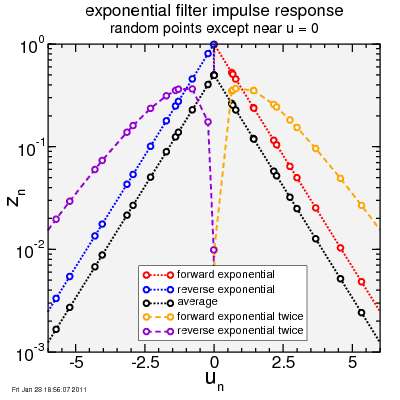
The x-axis is plotted versus my unitless normalized time variable u, which is the ratio of time to the time-constant of the exponential smoothing. The y-axis is then the filter response on a logarithmic scale.
Note despite the random spacing of points, the impulse responses follow smooth lines. For forward time, there is no response until the impulse hits, then the result exponentially decays from a maximum value. When the filter is applied twice in the forward direction, it no longer jumps instantly to the maximum value, but builds rapidly by continuously, then hits a peak, and fades from there. Reverse time, as expected, has the same shape as forward time but with the u-axis flipped. Given this, the result for averaging the forward and reverse time result is as expected: rising exponentially up, hitting a peak, then decaying exponentially down.
The Fourier transform of the impulse response of a linear filter is the filter's frequency response. If the goal is to smooth a function, you want the frequency response to drop off for high frequencies.
To test this, I created some new data, which were spaced at 0.01 intervals in u, again with an approximation to an impulse at zero. I ran the exponential filter twice in each case, as these generate the smoothest results without jumps: either twice in forward-time, twice in reverse time, or once in each direction. For the last option, I either averaged the forward and reverse directions applied in each case to the original data, or I ran forward direction to the original data then in the reverse direction on the smoothed result of the forward direction. I plot only the magnitude of the transform, not the phase:
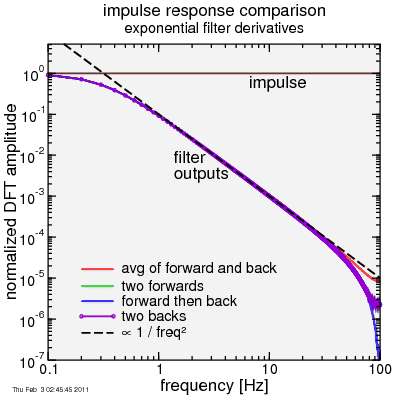
Start first with the impulse. The frequency response of a perfect impulse is a flat line. Since the transform was done with a discrete Fourier transform as opposed to a continuous Fourier transform, my approximation to a perfect impulse produces a flat result. Impulses have equal contributions from all frequencies.
Look then at the results of the filtered signals. Somewhat surprising, or maybe not, the frequency response in each case is almost the same: following a 1 / frequency-squared trend. In the case of applying an exponential filter twice, whether they differ in phase (which I'll show next), the magnitude of the frequency response is the same. The magnitude describes smoothness, while the phase describes delay, and while they have different degrees of delay, the smoothness is the same. Okay, there's some difference at the highest frequencies at the edge of the plot, but that's due to interpolation errors when applying the filter twice. The first exponential smoothing should result in an instant jump from zero, but since I interpolate between samples, there's some "leakage" into negative time for the forward-sweep, or positive time for the negative sweep. The averaged forward - reverse filter is less prone to this interpolation error.
Analytically the Fourier transform of an exponential convolution is about as simple as Fourier transforms get... the complex frequency response is:
F(ω) = 1 / [ i ω τ + 1 ]
where i is the unit imaginary number.
For the reverse direction, I flip ω → ‒ω :
F(‒ω) = 1 / [ ‒i ω τ + 1 ]
Each of these has the same magnitude:
|F(ω)| = 1 / sqrt[ω² τ² + 1 ]
So if I apply either twice I get a magnitude (since magnitudes of complex numbers multiply under multiplication):
|F(ω)²| = 1 / [ω² τ² + 1 ]
The phase, on the other hand, is:
φ[F(ω)] = ‒arctan[ωτ]
where φ specifies the phase, and arctan is the arctan. The sign flips on the phase for the reverse direction. If I apply a forward exponential twice, I therefore get double the phase (and therefore double the delay):
φ[F(ω)²] = ‒2 arctan[ωτ]
On the other hand, if I apply a forward followed by a reverse exponential, the phases cancel:
φ[F(ω)F(‒ω)] = 0
Zero phase is what we want: we want no time lag, just smoothing. So from a smoothing perspective, the double-forward or double-backward smoothing is the same as forward-backward. But from a delay perspective, the last option is the clear preference.
However, instead of doing forward then backward on the result (or vice-versa), I choose the average of the forward and backward. This results in a Fourier transform:
(F(ω) + F(‒ω)) / 2 =
[ 1 / [ i ω τ + 1 ] + 1 / [ ‒i ω τ + 1 ] ] / 2 =
1 / [ω² τ² + 1 ],
which is the same as the forward and reverse applied sequentially. Again the phase is zero (the imaginary part is zero). The advantage is in dealing with the first and the last point of the sequence, where the averaging approach is guaranteed to treat each end the same, but the sequential filter application can treat the end points differently.
Here's a plot of phases from a discrete Fourier Transform applied to my sample data (over 20 seconds with 100 points per second with an impulse approximated half-way):
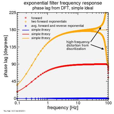
Things are behaving as expected from the equations out to extremely high frequencies where the "mesh" makes itself evident.
Okay, way too much on this, I suppose. The end result is taking the forward exponential smoothing, then the reverse exponential smoothing, results in a nice 1 / [ω² τ² + 1 ] low-pass filter without phase lag with the computational efficiency of exponential filtering. So that's what I use for altitude data.
‒0.01, 0
0, 100
0.01 0
I then ran this through my exponential filter in various ways.
One way is to run the points in time-forward order. This is the "causal" approach: I'm analyzing data as it comes, and I want a smoothed result as I am receiving data. Also causal is to run the smoothed curve again through the exponential filter. You'd expect this second smoothed result to be even smoother than the first time through, and of course it is.
Then there's a single and double application of the exponential filter in reverse time order. You'd expect the result to be flipped from the forward-time order (there's nothing special about forward time versus reverse time which should make the shape different; if it were there'd be something wrong).
As a third option, I do the filter in forward time and in reverse time, separately, and average the two results. This is very similar to running the filter for forward time and then running that smoothed result in reverse time.
Here's the results:
The x-axis is plotted versus my unitless normalized time variable u, which is the ratio of time to the time-constant of the exponential smoothing. The y-axis is then the filter response on a logarithmic scale.
Note despite the random spacing of points, the impulse responses follow smooth lines. For forward time, there is no response until the impulse hits, then the result exponentially decays from a maximum value. When the filter is applied twice in the forward direction, it no longer jumps instantly to the maximum value, but builds rapidly by continuously, then hits a peak, and fades from there. Reverse time, as expected, has the same shape as forward time but with the u-axis flipped. Given this, the result for averaging the forward and reverse time result is as expected: rising exponentially up, hitting a peak, then decaying exponentially down.
The Fourier transform of the impulse response of a linear filter is the filter's frequency response. If the goal is to smooth a function, you want the frequency response to drop off for high frequencies.
To test this, I created some new data, which were spaced at 0.01 intervals in u, again with an approximation to an impulse at zero. I ran the exponential filter twice in each case, as these generate the smoothest results without jumps: either twice in forward-time, twice in reverse time, or once in each direction. For the last option, I either averaged the forward and reverse directions applied in each case to the original data, or I ran forward direction to the original data then in the reverse direction on the smoothed result of the forward direction. I plot only the magnitude of the transform, not the phase:
Start first with the impulse. The frequency response of a perfect impulse is a flat line. Since the transform was done with a discrete Fourier transform as opposed to a continuous Fourier transform, my approximation to a perfect impulse produces a flat result. Impulses have equal contributions from all frequencies.
Look then at the results of the filtered signals. Somewhat surprising, or maybe not, the frequency response in each case is almost the same: following a 1 / frequency-squared trend. In the case of applying an exponential filter twice, whether they differ in phase (which I'll show next), the magnitude of the frequency response is the same. The magnitude describes smoothness, while the phase describes delay, and while they have different degrees of delay, the smoothness is the same. Okay, there's some difference at the highest frequencies at the edge of the plot, but that's due to interpolation errors when applying the filter twice. The first exponential smoothing should result in an instant jump from zero, but since I interpolate between samples, there's some "leakage" into negative time for the forward-sweep, or positive time for the negative sweep. The averaged forward - reverse filter is less prone to this interpolation error.
Analytically the Fourier transform of an exponential convolution is about as simple as Fourier transforms get... the complex frequency response is:
F(ω) = 1 / [ i ω τ + 1 ]
where i is the unit imaginary number.
For the reverse direction, I flip ω → ‒ω :
F(‒ω) = 1 / [ ‒i ω τ + 1 ]
Each of these has the same magnitude:
|F(ω)| = 1 / sqrt[ω² τ² + 1 ]
So if I apply either twice I get a magnitude (since magnitudes of complex numbers multiply under multiplication):
|F(ω)²| = 1 / [ω² τ² + 1 ]
The phase, on the other hand, is:
φ[F(ω)] = ‒arctan[ωτ]
where φ specifies the phase, and arctan is the arctan. The sign flips on the phase for the reverse direction. If I apply a forward exponential twice, I therefore get double the phase (and therefore double the delay):
φ[F(ω)²] = ‒2 arctan[ωτ]
On the other hand, if I apply a forward followed by a reverse exponential, the phases cancel:
φ[F(ω)F(‒ω)] = 0
Zero phase is what we want: we want no time lag, just smoothing. So from a smoothing perspective, the double-forward or double-backward smoothing is the same as forward-backward. But from a delay perspective, the last option is the clear preference.
However, instead of doing forward then backward on the result (or vice-versa), I choose the average of the forward and backward. This results in a Fourier transform:
(F(ω) + F(‒ω)) / 2 =
[ 1 / [ i ω τ + 1 ] + 1 / [ ‒i ω τ + 1 ] ] / 2 =
1 / [ω² τ² + 1 ],
which is the same as the forward and reverse applied sequentially. Again the phase is zero (the imaginary part is zero). The advantage is in dealing with the first and the last point of the sequence, where the averaging approach is guaranteed to treat each end the same, but the sequential filter application can treat the end points differently.
Here's a plot of phases from a discrete Fourier Transform applied to my sample data (over 20 seconds with 100 points per second with an impulse approximated half-way):
Things are behaving as expected from the equations out to extremely high frequencies where the "mesh" makes itself evident.
Okay, way too much on this, I suppose. The end result is taking the forward exponential smoothing, then the reverse exponential smoothing, results in a nice 1 / [ω² τ² + 1 ] low-pass filter without phase lag with the computational efficiency of exponential filtering. So that's what I use for altitude data.


Comments