smoothing Garmin altitude profiles for power estimation
Recall that I was contemplating using power in lieu of speed for determining whether a Garmin FIT file contains motorized segments. The speed criterion was fairly simple: if the data indicate the user got 500 meters ahead of a 14 m/sec pace over any segment, that segment was judged to be a portion of motorized travel. The entire region between load/unload opportunities was thus tagged and pruned. While cyclists may be able to sustain a high speed for short periods, by requiring they get a certain distance ahead of a threshold pace requires they exceed that pace for an extended time, or vastly exceed it for a shorter time.
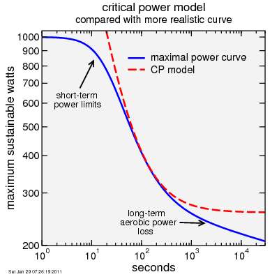
Example of critical power model applied to more realistic curve
In the power-time domain,the critical power model accounts for that ability to sustain high intensity for short times, but only a lower intensity for longer times. The critical power model is very similar to the criteria used for speed: it says a rider, given sufficient time, can do a given amount of work (the anaerobic work capacity, or AWC) above a critical rate of work production (the critical power, or CP). Taking a critical power typical of a world class cyclist in the golden era of EPO use, CP = 6.5 W/kg (normalized to body mass) makes a good threshold for suspicion of motorized assistance. A fairly typical AWC is 90 seconds multiplied by the critical power, so an AWC of near 0.6 kJ/kg would be applicable. Given these choices, if a rider can produce morethan 0.6 kJ/kg above 6.5 W/kg × Δt then the segment is judged to be motorized.
So we need a way to estimate power. We could use power meter data, but of course when a rider is in a car or train the power meter isn't registering. So instead we need to estimate power from the rider's speed and the altitude data. To provide a margin of error, we can make reasonably optimistic (low) assumptions about wind and rolling resistance. We then do as we did with speed: find data points where the rider crosses the 6.5 W/kg threshold, then look for segments connecting low-high and high-low transitions which are more than AWC above CP multiplied by the duration.
However, here's the rub: to estimate power at any given time we need to be able to estimate road grade. The iBike,for example, has accelerometers configured to directly measure grade,but with the Garmin Edge 500 you need to take differences of altitude and divide by differences in distance.
Unfortunately the Garmin is anything but smooth in its reporting of altitude versus time (and by implication versus distance). Here's some data measured on a stationary trainer... the altitude remains constant, then increases, then is constant, then increases. The jumps in altitude will tend to produce rapid spikes in the grade. So we need to smooth the data.
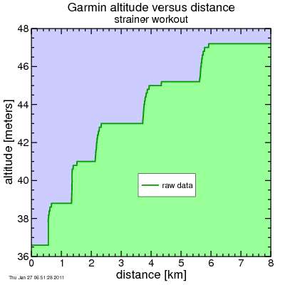
Garmin Edge 500 data from riding a trainer
So what sort of smoothing do we need? Assume the Garmin can jump ±1 meter at any time. If this happens over a 1-second interval, that's a rate of climbing of 1 meter per second, or 3600 meters per hour, which has a minimim energy cost of 9.8 W/kg (assuming the acceleration of gravity is 9.8 m/sec²). But the rider is likely lifting at least 1.15 kg/kg of body mass, and drivetrain efficiency is no better than 98%, so the actual cost of this climbing is closer to 11.5 W/kg. So every time the altitude jumped upward, we'd assume the rider blew past that 6.5 W/kg threshold. If I want to reduce the instantaneous error from this jump in altitude to be no more than 0.1 W/kg, a smoothing time constant of 120 seconds should do the trick, assuming an exponential convolution filter for computational efficiency.
So why is an exponential filter so computationally efficient? With an exponential filter, I calculate a running average. But instead of summing all of the samples which contribute to the average, I simply attenuate my sample I had for the previous point, and add in the component for the newest sample. I'm only processing one point per point. Consider instead the case with a convolution with another function, for example cosine-squared. With cosine-squared I need to sum the contribution from multiple points each time I move to an additional point. There's no way (at least no way I know) to reuse the sum calculated for the previous point.
For example, if I have points uniformly spaced in time with spacing Δt, and I have a smoothing time constant τ, and I want to go from an original time series yn to a smoothed time series zn as follows:
zn = zn‒1 exp(‒|Δt| / τ) + yn [1 ‒ exp(‒|Δt| / τ)]
It can't get much simpler than that. I'll revisit this formula later, as it has some weaknesses, in particular when data aren't uniformly spaced.
There's also the simple running average. Running averages can also be done efficiently, but they aren't so smooth. A point has no effect if it's outside the box, full influence if it's in. With an exponential average, a point has a sudden influence when it is first reached, but beyond that its influence slowly fades. I'll stick with exponential filters here.
More discussion next time.
Example of critical power model applied to more realistic curve
In the power-time domain,the critical power model accounts for that ability to sustain high intensity for short times, but only a lower intensity for longer times. The critical power model is very similar to the criteria used for speed: it says a rider, given sufficient time, can do a given amount of work (the anaerobic work capacity, or AWC) above a critical rate of work production (the critical power, or CP). Taking a critical power typical of a world class cyclist in the golden era of EPO use, CP = 6.5 W/kg (normalized to body mass) makes a good threshold for suspicion of motorized assistance. A fairly typical AWC is 90 seconds multiplied by the critical power, so an AWC of near 0.6 kJ/kg would be applicable. Given these choices, if a rider can produce morethan 0.6 kJ/kg above 6.5 W/kg × Δt then the segment is judged to be motorized.
So we need a way to estimate power. We could use power meter data, but of course when a rider is in a car or train the power meter isn't registering. So instead we need to estimate power from the rider's speed and the altitude data. To provide a margin of error, we can make reasonably optimistic (low) assumptions about wind and rolling resistance. We then do as we did with speed: find data points where the rider crosses the 6.5 W/kg threshold, then look for segments connecting low-high and high-low transitions which are more than AWC above CP multiplied by the duration.
However, here's the rub: to estimate power at any given time we need to be able to estimate road grade. The iBike,for example, has accelerometers configured to directly measure grade,but with the Garmin Edge 500 you need to take differences of altitude and divide by differences in distance.
Unfortunately the Garmin is anything but smooth in its reporting of altitude versus time (and by implication versus distance). Here's some data measured on a stationary trainer... the altitude remains constant, then increases, then is constant, then increases. The jumps in altitude will tend to produce rapid spikes in the grade. So we need to smooth the data.
Garmin Edge 500 data from riding a trainer
So what sort of smoothing do we need? Assume the Garmin can jump ±1 meter at any time. If this happens over a 1-second interval, that's a rate of climbing of 1 meter per second, or 3600 meters per hour, which has a minimim energy cost of 9.8 W/kg (assuming the acceleration of gravity is 9.8 m/sec²). But the rider is likely lifting at least 1.15 kg/kg of body mass, and drivetrain efficiency is no better than 98%, so the actual cost of this climbing is closer to 11.5 W/kg. So every time the altitude jumped upward, we'd assume the rider blew past that 6.5 W/kg threshold. If I want to reduce the instantaneous error from this jump in altitude to be no more than 0.1 W/kg, a smoothing time constant of 120 seconds should do the trick, assuming an exponential convolution filter for computational efficiency.
So why is an exponential filter so computationally efficient? With an exponential filter, I calculate a running average. But instead of summing all of the samples which contribute to the average, I simply attenuate my sample I had for the previous point, and add in the component for the newest sample. I'm only processing one point per point. Consider instead the case with a convolution with another function, for example cosine-squared. With cosine-squared I need to sum the contribution from multiple points each time I move to an additional point. There's no way (at least no way I know) to reuse the sum calculated for the previous point.
For example, if I have points uniformly spaced in time with spacing Δt, and I have a smoothing time constant τ, and I want to go from an original time series yn to a smoothed time series zn as follows:
zn = zn‒1 exp(‒|Δt| / τ) + yn [1 ‒ exp(‒|Δt| / τ)]
It can't get much simpler than that. I'll revisit this formula later, as it has some weaknesses, in particular when data aren't uniformly spaced.
There's also the simple running average. Running averages can also be done efficiently, but they aren't so smooth. A point has no effect if it's outside the box, full influence if it's in. With an exponential average, a point has a sudden influence when it is first reached, but beyond that its influence slowly fades. I'll stick with exponential filters here.
More discussion next time.


Comments